
Bilinear Interpolation Calculator
Instructions:
-
Review the methodology to ensure it aligns with your project's requirements.
-
Enter x1 and x2, which are the known bounding values for x
-
Enter x, which is the value for which you are interpolating
-
Enter y1 and y2, which are the known bounding values for y
-
Enter y, which is the value for which you are interpolating
-
Enter P11, P12, P21, and P22, which are the data points at (x1,y1), (x1,y2), (x2,y1) and (x,y2) respectively.
-
Click the Calculate button, and the interpolated value will be shown in Red in the center box.
Units are yours to choose: the four corner values P11, P21, P12 and P22 come out of a table in whatever units it is published in, and the result is in those same units. The x and y bounds only have to be consistent with each other.
The result is the weighted average of the four corner values, each weighted by the area of the rectangle diagonally opposite it, so the nearest corner counts for the most. It reduces to plain linear interpolation when x or y sits exactly on a bound.
Leave x2 blank to skip the x range check, or y1 blank to skip the y one. Otherwise the range check warns when x or y falls outside its bounds, where the formula extrapolates rather than interpolates.
Corrected 2026-09: the original's range check read the x2 and y1 boxes with a converter that did not recognise scientific notation, and anything it did not recognise dropped out of the comparison, leaving x or y checked against the opposite bound alone. Entering 1e3 for x2 therefore warned that a perfectly valid interpolation was out of range. The interpolation in the same table always read 1e3 as 1000, and so does Excel; both readings now agree.
Methodology, Equations & Example:
This Bilinear Interpolation Calculator returns an interpolated value based on the bilinear interpolation algorithm. The term "bilinear" refers to an interpolation technique that considers the values of the four nearest neighboring data points to estimate the value of a point within the grid. These four points form a square, and the interpolation calculates the weighted average of their values based on the distance from the desired point. In addition to "bilinear interpolation," this technique may also be referred to as "double interpolation" or "bi-linear filtering" in certain contexts.
Bilinear interpolation is performed by considering the distances of the desired point from each of the four nearest pixels. The distances are used to calculate weighting factors, which determine the contribution of each pixel to the interpolated value. The closer a pixel is to the desired point, the higher its weight. Once the weights are determined, they are multiplied by the corresponding point values and summed to obtain the interpolated value.
The method of Bilinear Interpolation or double interpolation is as follows:
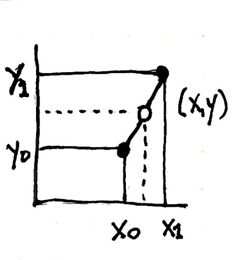
Step 1 Perform a linear interpolation at point (x,y1):
R(x,y1) = P11(x2-x)/(x2-x1) + P21(x-x1)/(x2-x1)
Step 2 Perform a linear interpolation at point (x,y2):
R(x,y2) = P12(x2-x)/(x2-x1) + P22(x-x1)/(x2-x1)
Step 3 Perform a linear interpolation at point (x,y) using the results from Step 1 and Step 2:
R(x,y) = R(x,y1)(y2-y)/(y2-y1) + R(x,y2)(y-y1)/(y2-y1)
Step 4 Substitute values for R(x,y2) and R(x,y2) to find the resulting interpolated value, R(x,y), at point (x,y):
R(x,y) = P11(x2-x)(y2-y)/((x2-x1)(y2-y1)) + P21(x-x1)(y2-y)/((x2-x1)(y2-y1)) + P12(x2-x)(y-y1)/((x2-x1)(y2-y1)) + P22(x-x1)(y-y1)/((x2-x1)(y2-y1))

Example:
Suppose you want to calculate the Total Cooling Capacity of a 5-ton Bryant® package unit. A snippet of the equipment's performance data table at design conditions is provided. For our scenario, the design conditions are:
-
Condenser Entering Air Temperature: 79oF
-
Evaporator Entering Wet Bulb Temperature: 65oF
Solution:
This example will be solved three times. Solution 1 will be to perform linear interpolation three times using Steps 1, 2, and 3 above. Solution 2 will use the combined bilinear interpolation equation shown in Step 4 above. Solution 3 will show how to use the calculator to obtain the results.
For all solutions, the following inputs are below as provided in the table or given values:
P11 = 55.04 MBtuh
P12 = 59.00 MBtuh
P21 = 52.59 MBtuh
P22 = 56.34 MBtuh
x1 = 75oF
x2 = 85oF
y1 = 63oF
y2 = 67oF
x = 79oF
y = 65oF

Solution 1:
Step 1: Interpolate around point (x,y1)
R(x,y1) = P11(x2-x)/(x2-x1) + P21(x-x1)/(x2-x1)
= 55.04 (85-79)/(85-75) + 52.59 (79-75)/(85-75)
= 54.06 MBtuh
Step 2: Interpolate around point (x,y2)
R(x,y2) = P12(x2-x)/(x2-x1) + P22(x-x1)/(x2-x1)
= 59.00(85-79)/(85-75) + 56.34(79-75)/(85-75)
=57.936 MBtuh
Step 3 Perform a linear interpolation at point (x,y) using the results from Step 1 and Step 2:
R(x,y) = R(x,y1)(y2-y)/(y2-y1) + R(x,y2)(y-y1)/(y2-y1)
= 54.06(67-65)/(67-63) + 57.936(65-63)/(67-63)
=55.998 MBtuh
Solution 2:
The bilinear interpolation as a single equation as shown above:
R(x,y) = P11(x2-x)(y2-y)/((x2-x1)(y2-y1)) + P21(x-x1)(y2-y)/((x2-x1)(y2-y1)) + P12(x2-x)(y-y1)/((x2-x1)(y2-y1)) + P22(x-x1)(y-y1)/((x2-x1)(y2-y1))
R(x,y)=55.04(85-79)(67-65)/((85-75)(67-63))+52.59(79-75)(67-65)/((85-75)(67-63))+59.00(85-79)(65-63)/((85-75)(67-63))+56.34(79-75)(65-63)/((85-75)(67-63))
=55.998 MBtuh
Solution 3: To Solve using the calculator, enter the inputs in the same order that they appear in the table. Below is a table showing the inputs. The result is shown in red in the middle of the table as 55.998MBtuh.
